Parallelizing LLMs
Important link to understand GPU sync operations: https://docs.nvidia.com/deeplearning/nccl/user-guide/docs/usage/collectives.html
Data Parallelism
Naive data parallelism - HF accelerate / PyTorch DDP
Eg: Split batch-size and split into machines - calculate gradient - exchange gradients to sync
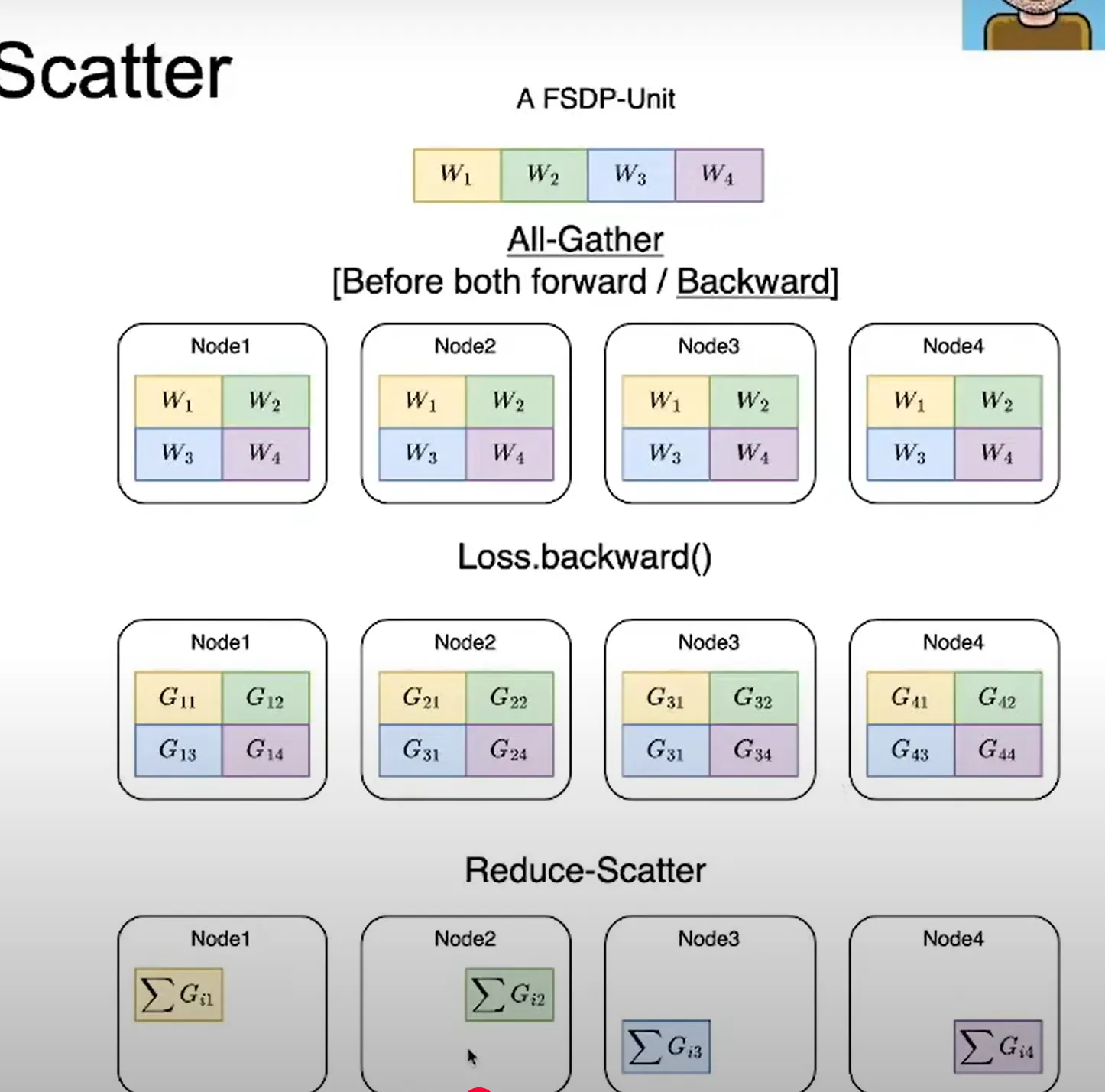
- All reduce operation = Reduce-scatter (occurs first) + All-gather (occurs next)
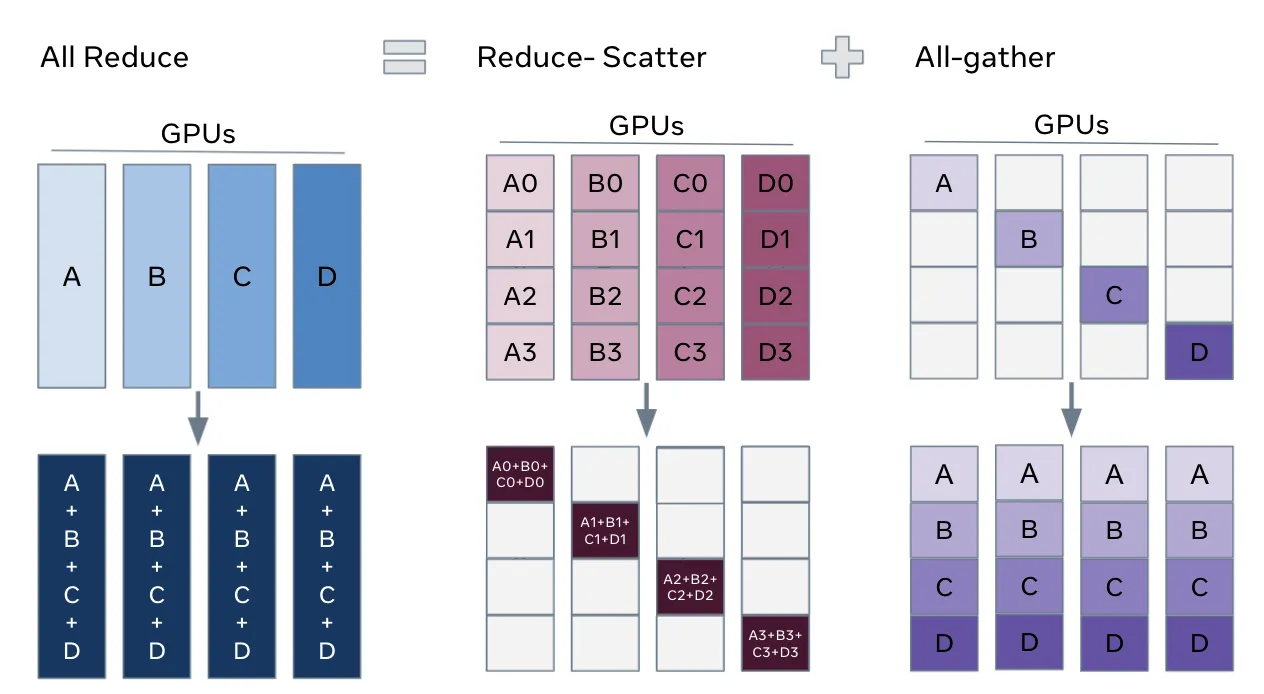
- Computer scaling - GPU: B/M examples (can saturate compute since each gpu has decent micro batch size) - B/M: batch by microbatch
- Communication overhead - 2x number of params every batch since we do reduce-scatter then all-gather (fine for bigger batches - overhead of synch gradients)
- Memory scaling - none - every gpu has to replicate optimizer state and num params so not good from memory point of view → big bottleneck since we duplicate over gpu.
**Optimizer states are memory heavy** - stores state corresponding to parameters (eg: momentum buffer), param groups with lr, weight decay, param_ids, etc.
Zero 1-3: Distributed data Parallel
Do we need optimizer state, every gradient, and every parameter calc on every machine? → can be sharded
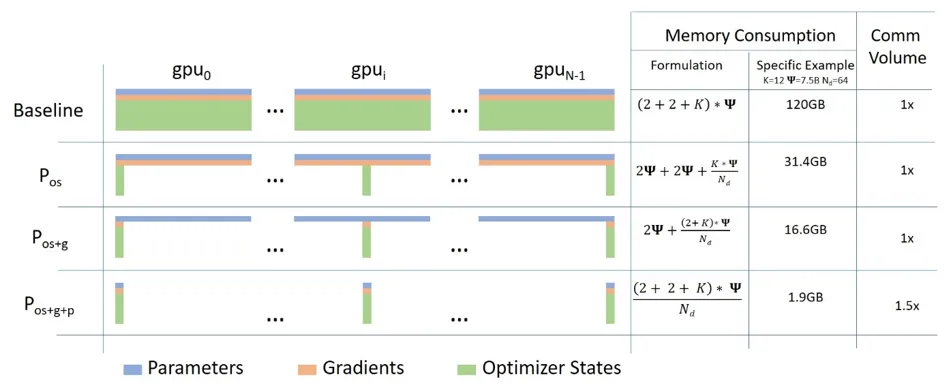
Stage 1: Optimizer State Sharding
- Everyone has gradients and parameters → calculates everything
- Optimizer states is split: Optimizer state contains https://docs.pytorch.org/docs/stable/generated/torch.optim.Optimizer.state_dict.html
- Reduce scatter the gradient: incurs #param comm cost
This way GPU 0 gets all gradient info from all other GPU for subset of params it is responsible for. - Each machine updates their params
- All gather updated params: incurs #param comm cost
- 2x #param comm cost since we are communicating each set of params to each of the machines
- Memory constraint is divided by number of GPU for the number of optimizer GPUs: Linear scaling
Stage 2: Extension to Gradient Sharding
- Full param, sharded gradients and sharded optimizer state
- We never instantiate a full gradient vector - so everyone incrementally goes backward on computation graph
- Immediately reduce gradient → send to a worker, once gradients aren’t needed → immediately free it
- Each machine updates their own parameter using gradient plus opt state
- All gather the updated params (since only chunks of params are updated in each machine)
- Minimal overhead even though more communication
Stage 3: FSDP - Shard Params too
- send and request params on demand
- Incremental communication and computation
- Relatively low overhead
- Performs repeated all-gather and free-weights
- However, activation memory is stored for the backwards
- Backward pass is all-gather and reduce scatter again → update the model, splits params and frees full weights
- Total communication cost is higher - 3x #param comm cost + waiting
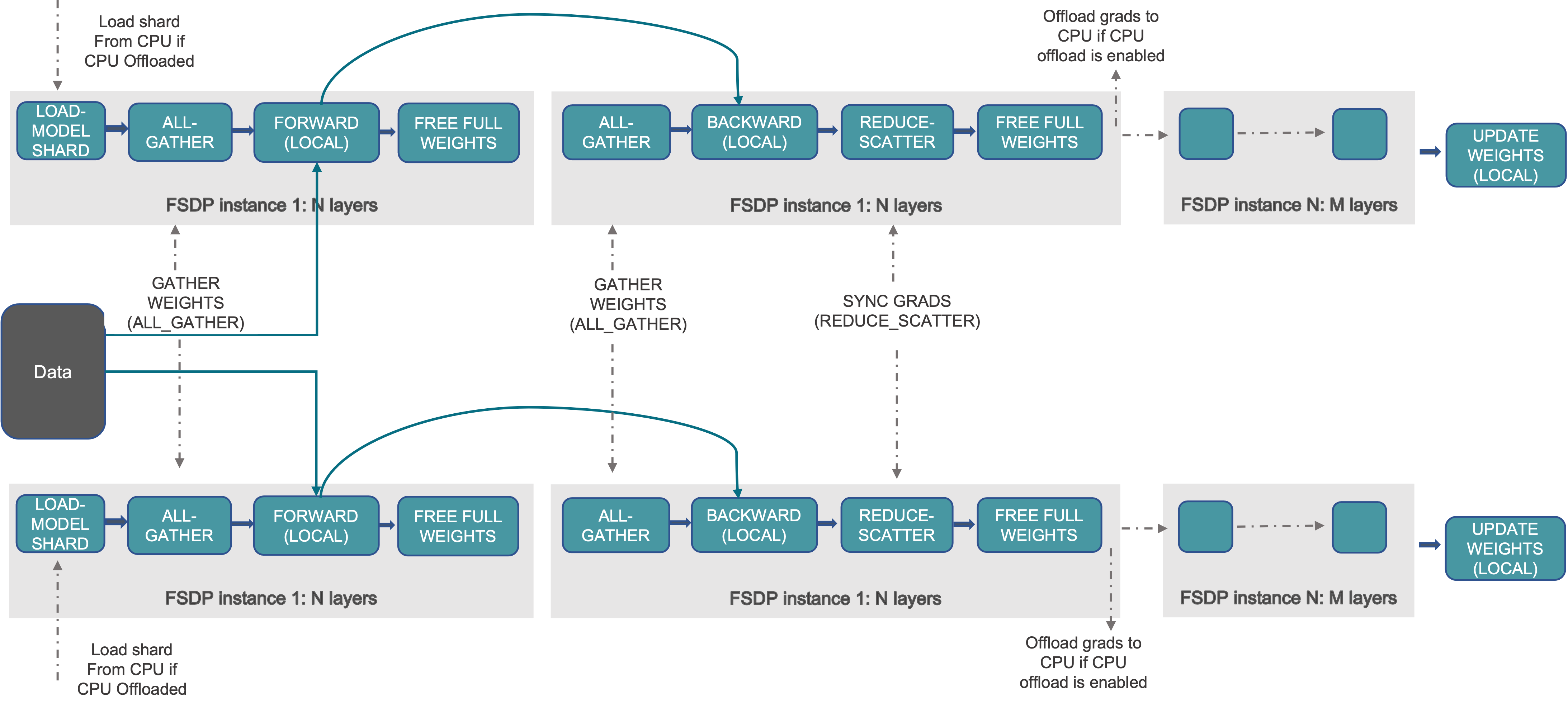
- Load shard – each rank loads its shard of parameters (GPU or CPU→GPU if offloaded).
- All-gather weights – gather full parameters for the current layer block (only for the current block to process forward pass).
- Forward (local) – run forward pass on local data.
- Free full weights – discard full params, keep only shard.
- All-gather weights (again) – before backward for that block.
- Backward (local) – compute gradients.
- Reduce-scatter grads – sum gradients across ranks and keep only each rank’s shard.
- Free full weights – free gathered params.
- (Optional) offload grads – move grad shards to CPU.
- Optimizer step (local) – update only the local parameter shard.
- The block distinction is important for fsdp block / layer optimization or selection. If we do zero3, assuming that we dont have a particular partition like in fsdp, then, as we go down the layers, shards of parameters all-gathered (eg: all-gather only p1, then free, then all-gather p2, free, so on..). The same concept is applied to fsdp but we think in terms of layers or blocks then [to reduce idle time, etc.]
- But, have overlapping communication and computation - all gather happens all at once when forward pass happens - masking some of the comm costs.
Communication and Computation for (W1W0 + W2W0)x = y
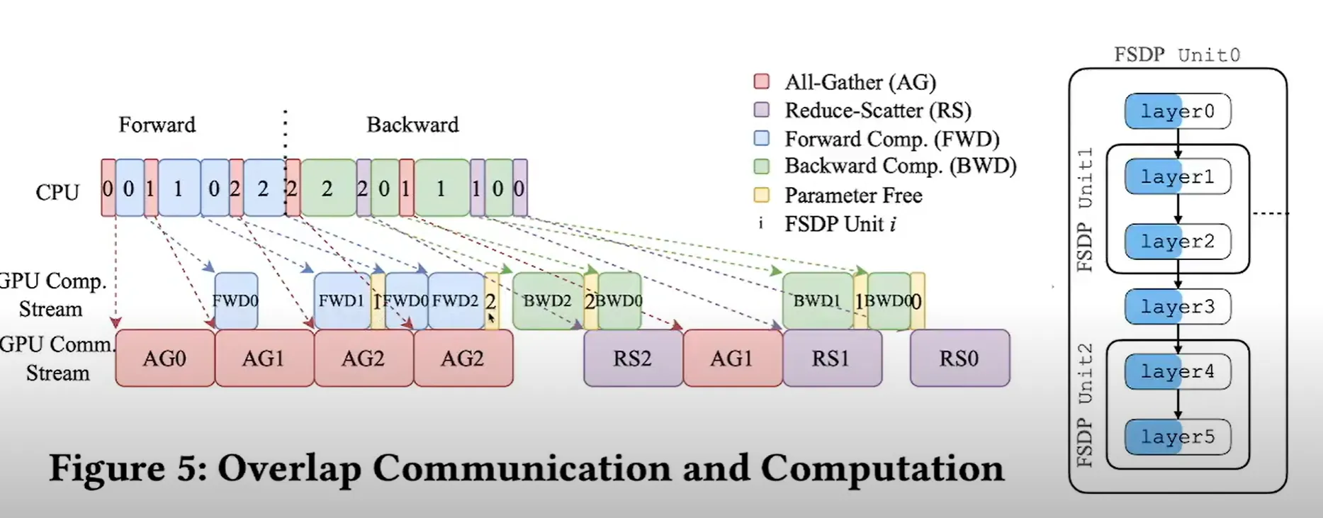
Forward
- All-gather params for unit 0 (AG0) while CPU preps next shards
- Forward compute unit 0 (FWD0)
- Free unit 0 params
- All-gather unit 1 (AG1) overlaps with FWD0
- FWD1 → free, then AG2 → FWD2 → free
→ repeat per FSDP unit
Backward
6. Backward unit 2 (BWD2)
7. Reduce-scatter grads for unit 2 (RS2) overlaps with next BWD
8. BWD1 → RS1, then BWD0 → RS0
9. Free params after each unit, optimizer updates local shards
FSDP Units:
Layers are sharded across the GPUs so that idle time between the GPUs can be reduced (compared to splitting say, Layer0 in GPU0, 1 in GPU1, 2, in GPU2)
Horizontal Sharding (Parameter-wise)
shard rows
- Method: Flatten all model parameters into a 1D tensor, then split into equal chunks across ranks
- Distribution: Each rank owns the same "slice position" across all layers
- Processing: All ranks work on the same FSDP unit simultaneously
- Benefit: Better load balancing, parallel processing
- Main cost: activation traffic between stages + pipeline bubbles
- Split by layers / modules
- Each GPU owns entire layers
- Used by pipeline / model parallelism
- Activations move between GPUs
Vertical Sharding (Layer-wise)
shard columns
- Method: Group layers into FSDP units (can be non-consecutive layers like 0,3 vs 1,2)
- Distribution: Different ranks own different FSDP units
- Processing: Must follow dependency order during forward/backward, but grouping is flexible
- Benefit: Less communication overhead, good for very deep models
- Main cost: weight all-gathers + grad reduce-scatters
- Split within a tensor
- Each GPU holds a slice of every layer
- Used by ZeRO-2 / ZeRO-3 / FSDP
- Needs all-gather to reconstruct full params
All Gather the layer sharded across GPUs (i.e. Layer0 across gpus) → forward pass
(Note: This is used in conjunction with DDP)
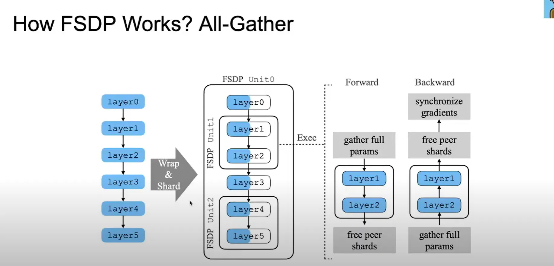
By processing one FSDP unit at a time:
- Only need parameters for the current unit in GPU memory
- Can free parameters from previous units (shown in yellow "Parameter Free" regions)
- Dramatically reduces memory requirements compared to keeping all model parameters loaded simultaneously
- CPU communicates commands - moves faster than the GPU does
- Load/gather and compute can happen overlapping
- Each machine has the activations to be able to perform next operation basically (hence the all-gather)
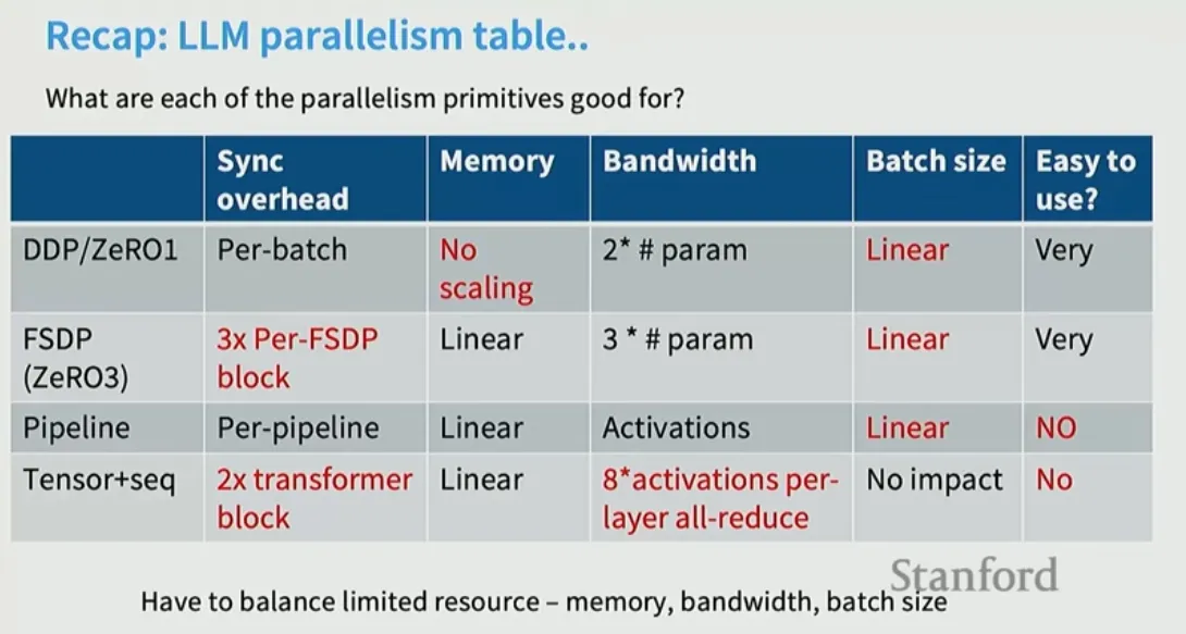
Issues with Data Parallelism:
- Batch size is important → num batches need to be more than num machines (Global batch size = per-GPU batch × #GPUs × grad accumulation)
- Past a certain point, huge batch sizes don’t offer much important
- Data parallelism alone can’t reach us to full potential of parallelism
- Does not reduce activation memory
Model Parallelism
Scale memory without changing batch sizes by splitting params across gpus but also communication activations
The focus on this type of parallelism is on the parameters. Activations are still a bottleneck.
Pipeline Parallel
Layer wise parallel - each GPU is assigned a layer and activations and gradients are passed around. Most GPUs are idle each time** since they need to wait between compute and communication.
Key notions:
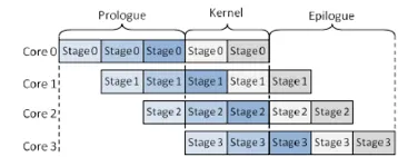
- Prologue (warm-up): The initial period when the first few microbatches are entering the early stages while later stages are still idle. This creates an initial “bubble.”
- Steady state: Once the pipeline is filled, each stage works on a different microbatch concurrently. This is where throughput is highest.
- Epilogue (drain): After the last microbatch enters the first stage, stages begin to go idle from the front to the back as the pipeline drains. This creates a final “bubble.”
- Pipeline bubble: The idle time due to prologue and epilogue. With p pipeline stages and m microbatches, an upper-bound efficiency for a simple Pipe-style schedule is approximately: efficiency ≈ m/[m+(p−1)]
Increasing microbatches m shrinks the relative bubble but raises activation memory. Interleaving (virtual stages) and better schedules can help.
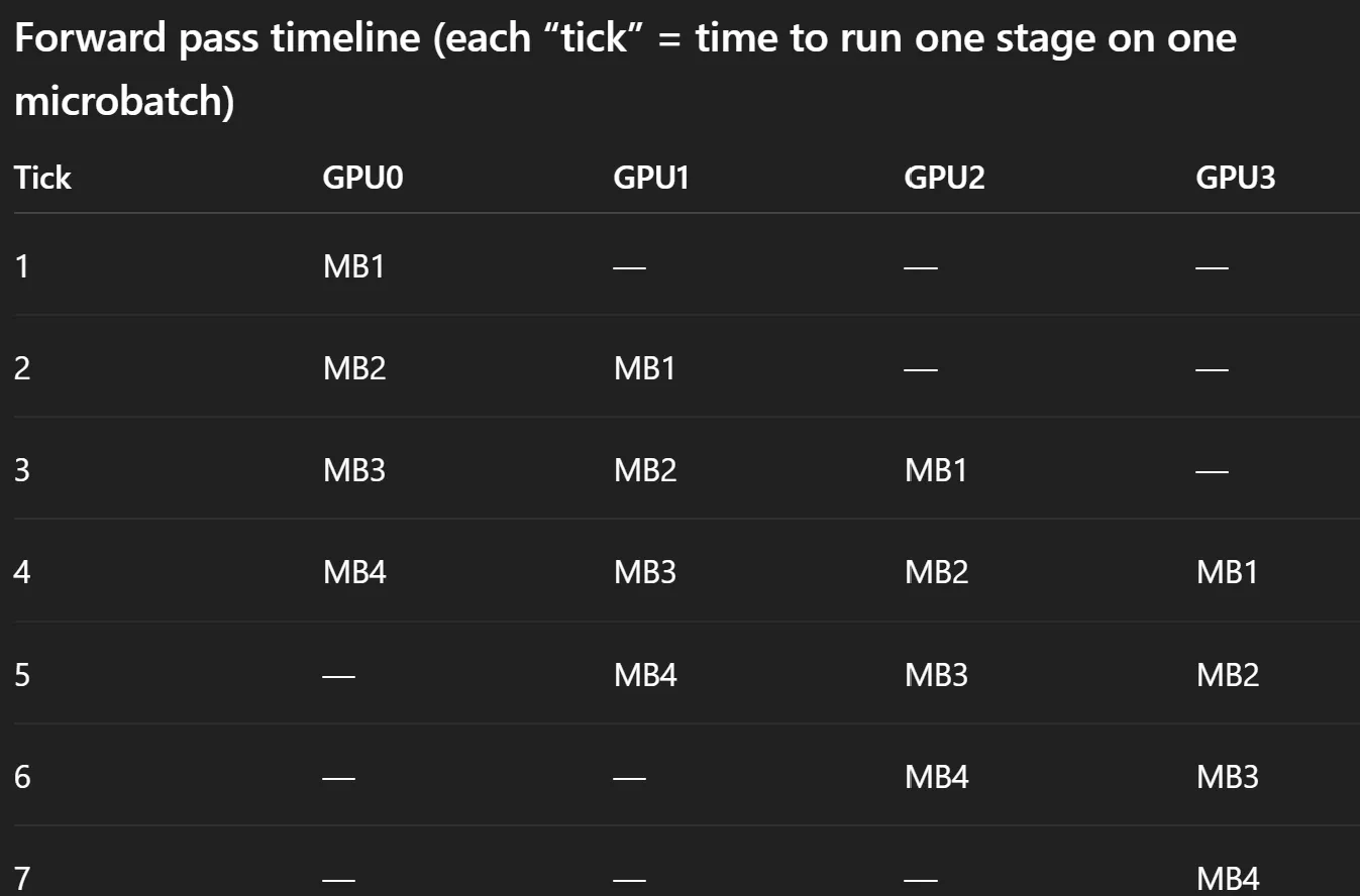
Pipeline parallel tries to ensure the wait time is reduced
- Have micro batches - process on a micro batch → send info to next gpu and start processing next micro-batch : reduces wait by having overlap in processes. Bubble time is controlled this way.
- But, batch sizes are finite - unless huge batch size - hard. This parallelism is highly dependent on batch sizes
- Help save more memory since it also shards activations
- Can be good for slower network lengths since it is point to point.
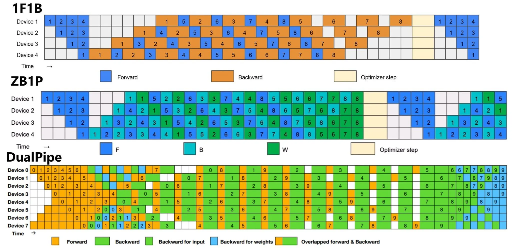
- Research exists on different pipeline interleaving to improve bubble time
- ZB1P = zero bubble, Dual Pipe
Reschedule pipeline to calculate update weights and perform updates such that we can further reduce the amount of time spent idle - Very complicated - requires intervening at Autograd, queues, etc.
- Avoided in training sometimes due to complexity as well as communication overheads: Inter-stage transfers for activations and gradients add latency; this interacts with DP/optimizer sharding (e.g., ZeRO/FSDP) and can complicate step-time
Difference between FSDP and Pipeline Parallelism and why pp is model parallelism over data parallelism
- DP/FSDP: GPUs work on different data and then globally sync gradients (all-reduce / reduce-scatter).
- Pipeline: GPUs work on different microbatches and pass activations/gradients along the chain (neighbor sends/recvs), plus you may optionally add DP on top.
Tensor Parallel
Think of cutting along the width → parallelizing and decomposing matrix multiplies by splitting into sub-matrices and partial sums.
Tensor parallelism splits a single layer’s math across multiple GPUs by slicing its tensors (weights, activations) along a dimension. Unlike data parallelism where whole model is split across gpus and work on different batches, here the GPUs operate on the same batch so computation is split on the GPUs.
Column-parallel (split outputs)
Split W by columns: W = [W₀ | W₁ | … | W_{P−1}], each of shape [d_in, d_out/P]. Every GPU holds the full input x and its own W shard and computes its shard of the output:
- On GPU p: y_p = x W_p (shape [batch, d_out/P])
The output y is sharded by feature dimension across GPUs. If the next op needs the full y on each GPU, you would all-gather the shards. If the next op can accept the sharded y, you skip that collective.
When it’s handy: the first MLP projection in a Transformer often expands H → 4H; column-splitting means each GPU computes a disjoint chunk of those 4H features entirely locally.
Row-parallel (split inputs)
Split W by rows: W = [W₀; W₁; …; W_{P−1}], each of shape [d_in/P, d_out]. Split the input x the same way: x = [x₀ | x₁ | … | x_{P−1}] along the feature dimension. Every GPU computes a partial output and then you sum across GPUs:
- On GPU p: p_p = x_p W_p (shape [batch, d_out])
- Then y = Σ_p p_p via an all-reduce (sum) so that every GPU gets the full y
The output is replicated after the collective. If you don’t need a fully replicated y, you can reduce-scatter instead to keep y sharded.
When it’s handy: the second MLP projection 4H → H; splitting rows lets each GPU multiply its local 4H/P activations with its weight rows and then one sum combines results.
The useful combo: column then row to avoid an extra collective
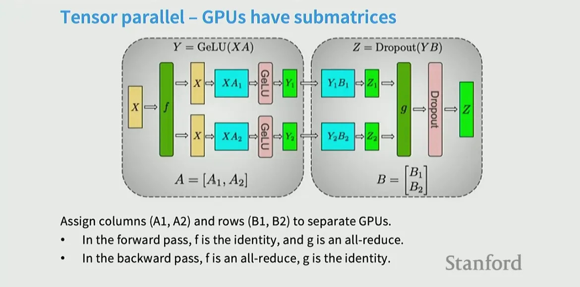
A classic Transformer MLP block is:
x → Linear(H → 4H) → GeLU → Linear(4H → H)
If you do:
- First linear as column-parallel: each GPU computes its shard of 4H features, no collective needed.
- Keep that shard local through GeLU (elementwise, no comm).
- Second linear as row-parallel: each GPU multiplies its local 4H/P slice, then a single collective at the end combines partial outputs.
Result: the pair of linears uses only one collective (at the end). If instead you had gathered after the first linear to assemble full 4H before the second, you would pay for an all-gather plus an all-reduce. Pairing column-parallel followed by row-parallel eliminates the all-gather.
Biases and dropout/activation are applied locally to each shard. (element wise operations)
Residual adds may require aligning shard layouts; see “sequence parallelism” below.
- f and g are synchronization barriers (they are the collective functions)
- This is expensive though since it needs to communicate a residual activation twice - forward backward [i.e. in the instance that collective is required]
- Hence - tensor parallel is applied in the same box or node that are connected with very fast connection since it is a bandwidth expensive process.
- Compared to pipeline parallel - don’t have to think of bubble
- Relatively low complexity - need to identify where largest matrix multiplies exist
- Doesn’t require large batch sizes to work well
- Disadvantage is large communication overhead and hence is used only in places that allows for high speed communication.
- Column-parallel layers require each GPU to hold the full input activation, increasing total activation memory across the TP group. If you later all-gather outputs to switch layouts, peak activation memory spikes.
- Small shards can also reduce efficiency by underutilizing tensor cores (that are shape dependent).
Both tensor parallel and pipeline parallel can be used simultaneously
Usually, tensor parallel applied first for the larger computations
Tensor parallel within machines and a combo of pipeline parallel and data parallel across machines → pipeline parallel mostly useful if model doesnt fit within machines with ease
→ 3D parallelism: Tensor parallelism + pipeline parallelism + data parallelism
Activation Parallelism
Activation memory continues to grow since some parts of it don’t parallelize cleanly
Recomputation helps keep activation memory low
• Gradient checkpointing → Saves memory during training. Instead of keeping all intermediate activations for backprop, it only saves a few “checkpoints” and recomputes the missing activations on the fly during backward pass. Trade-off: less memory, more compute.
Activation memory required per layer = sbh (34 + 5as/h)
S = seq Len, h = hidden dim, a = attn heads
LHS term from MLP, RHS term - attn
Tensor parallel can help but we have terms that will grow with size - that are non matmul terms
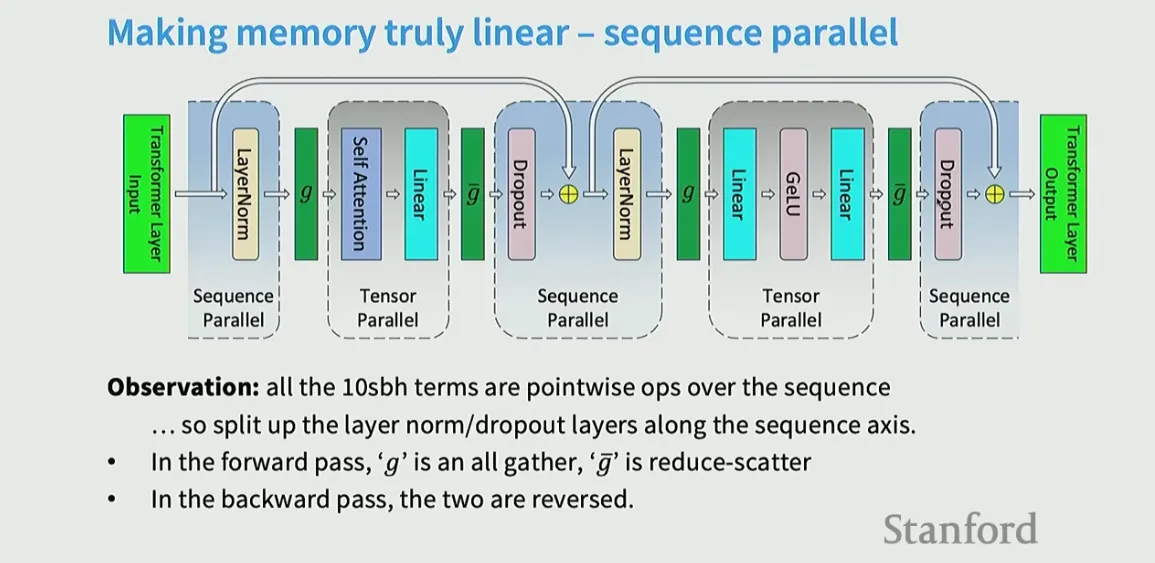
Sequence Parallel / Context Parallel
Making memory truly linear - Goal: reduce activation memory (and sometimes extend context length) by splitting the sequence dimension across devices, typically alongside tensor-parallel sharding of model weights.
- splitting up non-matmul operations to ensure we curb the activation memory growth for these
- So, split layer norm / dropout across sequence axis - layer norms don’t interact across positions of the sequence so each device can now handle one part across the sequence dimensions and then we sync them → no intercomm required, reducing or eliminating global gathers
- With sequence parallelism over g GPUs, each holds roughly [B, S/g, H] activations.
- Activation memory drops roughly by a factor of g for sequence-sharded tensors. That is often the largest memory consumer in long-context models.
- It composes well with tensor parallelism (sharding H) and with ZeRO/FSDP (sharding optimizer states), enabling very long sequences without OOM.
- The communication overhead for aggregating these partitions can be substantial, negating some of the benefits of parallelism.
- With sequence sharding, you must all-gather or ring-pass K/V (or attention outputs) across devices every step, adding per-token latency that’s hard to hide with small batches.
- Small-batch inefficiency. Inference often runs with batch size 1–8. Collectives and ring-passing benefit from larger batches; at small batch sizes their overhead dominates, increasing time-to-first-token and time-per-token
- Sequence/context parallelism is excellent for training and for prefill of very long sequences, but for interactive autoregressive decoding it usually increases latency and complexity due to per-token cross-device communication and KV-cache sharding.
- For most latency-sensitive inference, prioritize tensor parallelism, careful batching, and possibly hybrid approaches (multi-GPU prefill, single-GPU decode) before resorting to sequence sharding.
Context Parallelism (CP):
- Also distributes the sequence dimension across GPUs.
- Extends sequence parallelism by parallelizing the attention mechanism itself.
- This means that the computation for attention, which involves interactions between different parts of the sequence, is also distributed.
- CP is particularly useful for very long sequences, as it can reduce both memory and computation costs.
In essence:
- Sequence parallelism focuses on splitting the sequence for processing across layers.
- Context parallelism builds upon sequence parallelism by also distributing the attention mechanism itself.
- Context parallelism is a tailored variant for attention and KV-cache that replaces large, blunt all-gathers with streamed/ring-style exchanges of K/V (and sometimes partial attention outputs), improving overlap and memory behavior. Think: “sequence sharding with attention-aware communication.”
Concretely, for a microbatch of shape [B, S, H] split across g GPUs along S, each GPU holds roughly [B, S/g, H] tokens. The challenge is enabling each query to see keys/values from all shards without materializing the entire sequence on each device.
How attention works under CP
Two key phases have different patterns:
- Prefill (encoding a prompt of length S0):
- Goal: compute full self-attention over the prompt, filling the KV cache.
- Pattern: ring or staged all-gather of K/V blocks. Each GPU computes local Q/K/V for its token slice, then circulates K/V blocks to neighbors in g steps. At step t, a device attends its local Q against the currently held K/V block, accumulating partial softmax numerators and denominators. Use online/streaming softmax to remain exact without storing full logits.
- Memory: you never allocate [B, S0, H] on a single GPU; you stream blocks and keep running softmax stats.
- Communication: O(g) stages per layer per prefill. With NVLink/NVSwitch and good overlap, throughput stays high for long prompts.
- Decode (autoregressive generation, one or few tokens per step):
- Goal: each new query at position S0 + t must attend to all prior K/V in the cache.
- KV-cache sharding: each device stores its shard of the cache (roughly [B, S0/g, Hk] for K and [B, S0/g, Hv] for V per head).
- Per-token step: devices compute local K/V for the new token and insert them into the local shard; then they exchange either the new K/V or partial attention contributions so every query can incorporate all history. Implementations typically:
- Send the new K/V to all shards (all-gather small per-step tensors), or
- Keep new K/V locally and perform a ring across shards of the cached K/V blocks to compute attention contributions, similar to prefill but now only for the current query.
- Latency: there is unavoidable per-step communication across g shards; batching can amortize, but small-batch latency increases with g.
Add img
Collectives and kernels
- Streaming/ring attention: passes K/V blocks around the ring, fusing matmul + partial softmax reduce into each step to avoid large intermediate tensors.
- Online softmax: maintains running max and sum for numerical stability when accumulating across shards.
- Reduce-scatter / all-gather on the sequence dimension: used to keep outputs sharded after attention or to restore contiguous layouts when needed.
- Fused token permutation: when used with MoE or packed batches, CP often requires efficient gather/scatter of token blocks to avoid framework overhead.

Expert Parallelism:
NVLink
NVLink is a high-speed GPU-to-GPU interconnect technology developed by NVIDIA that offers significantly faster data transfer than traditional PCIe-based solutions. It enables multi-GPU systems to scale memory and performance for demanding visual computing and AI workloads by providing direct, high-bandwidth communication between GPUs. The technology, including the NVLink Switch, allows for powerful, interconnected GPU clusters used in high-performance computing (HPC) and data centers.
Other good resources:
https://docs.nvidia.com/nemo/megatron-bridge/0.2.0/parallelisms.html