Diffusion

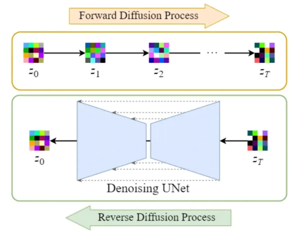
Image + Gaussian Noise → multiple times to achieve sample of pure noise.

Then, reconstruct from noise to retrieve image.

Forward process pushes a sample off the data manifold whereas the reverse process tries to push it back, close to its original position in the data manifold

Forward Diffusion

• Image from train set ⇒ x0
• Gradually add noise.
• Distribution of next time step only depends on its immediately previous time step (Markov chain) → successive single step conditions
• Continuous data → each transition parameterized = diagonal Gaussian, variance at time t = beta (usually hyperparam, increases over time, non-zero <1, brings mean of each new gaussian closer to 0)
• As T→ inf, q → Gaussian centered at 0 (identity covariance) i.e. as time goes on → modeled as perfect Gaussian noise (q here, is the forward process representation). At this point, lose all info of original samples.
• In practice, T is in order of 1000s, large steps, allow Beta to be small
• Benefit of small step size: gets easier to undo process.
  We want to determine, where did the chain come from (posterior) to arrive at x(t). If q(x(t)|x(t-1)) is large step, more ambiguity / uncertainty of x(t-1). Makes it easier to model gaussian

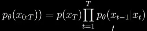
Reverse Diffusion

• True reverse process has same functional form as forward process (esp. with infinitesimally small steps).
• So, p i.e. reverse process, is parameterized to be a unimodal diagonal gaussian
• It takes in t as input to account for forward process variance schedule, so model learns to undo individually
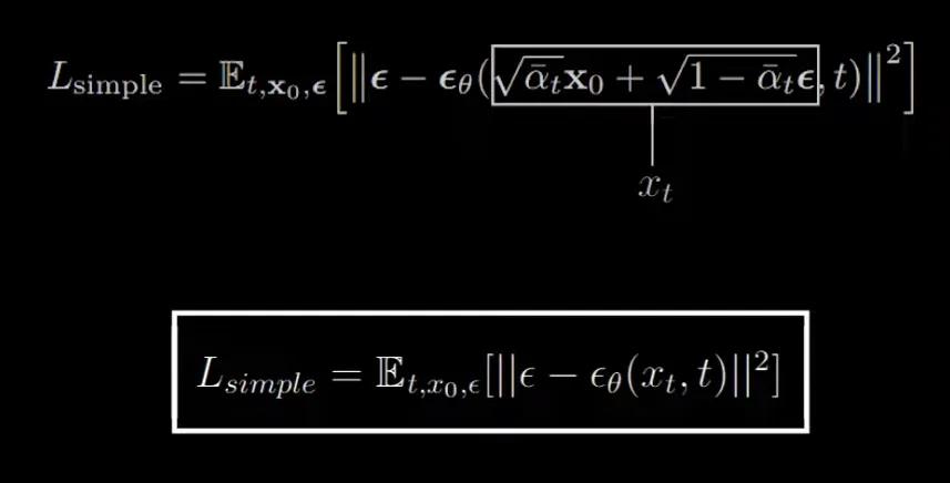
• Reparameterized to predict noise rather than mean or the image pixel.

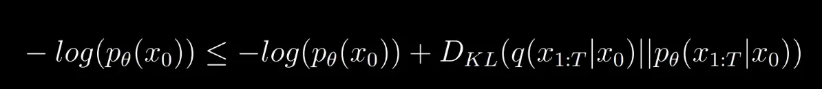
If we want to model x0, marginalize or integrate over all the different ways or trajectories we could reconstruct, but this is intractable, but, a lower bound can be estimated. Since it’s not tractable, we have to go step-wise, and cant denoise all at one step.

The sum of independent Gaussian steps is still a Gaussian

i.e., any arbitrary step of the forward process can be sampled directly in closed form. So during training time, any term of forward pass can be obtained without simulating a chain.

Diffusion sample can be trained conditionally. There have been work where diffusion process has been guided by trained classifier with the direction of gradient from the classifier. But, need second network. But, papers have shown classifier free diffusion guiding. Here, conditional label is set to null label with some probability during training and during inference, reconstructed sample are artificially pushed towards y and away from null label. No new info given to model but, had higher performance.

Paper 1: DDPM

1 and 3 are just different parameterizations of one another

Amount of noise added at each time step regulated by a schedule that is based on scaling the mean and variance, so that variance doesnt explode over time. Paper implements simple linear schedule

U-Net architecture with attention block at certain resolutions + ski connections between upsample and downsample

Time step - via sinusoidal embedding, to know how much noise to remove at diff timestep (since scaled by mean and variance)

Paper 2: OpenAI Improved DDPM

2. Found regulated noising be suboptimal (last few timesteps redundant - already reach approximation) + believe linear schedule leads to faster deterioration / loss of information of image - propose cosine scheduling to tackle

Math

$x_t$ Image at time step t.

$x_T$ image at last step T.

Forward process $q(x_t|x_{t-1})$ Reverse process $p(x_{t-1}| x_t)$

Forward diffusion process

$q(x_t|x_{t-1}) = \Nu(x_t, \sqrt{1-\beta_t}x_{t-1}, \beta_tI)$ Normal dist(output, mean, variance) $\beta_t \in (0,1)$ fixed value

$\alpha_t = 1-\beta_t; cumulative(\alpha_t) = mul(\alpha_s)$

“A property of Gaussian distributions, where the variance of the sum of two independent Gaussian variables is the sum of their variances.”

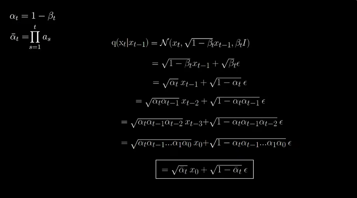
Basically refers to the point before “i.e., any arbitrary step of the forward process can be sampled directly in closed form. So during training time, any term of forward pass can be obtained without simulating a chain.”

Reverse diffusion process

$p(x_t|x_{t-1}) = \Nu(x_{t-1}; \mu_\theta(x_t, t), \Sigma_\theta(x_t, t))$ Now, variance here is fixed to certain schedule (DDPM), just have to learn mean.

Loss function = $-log(p_\theta, x_0)$ but $x_0$ depends on all subsequent time steps variables → cant keep track of that. Solution: compute variational lower bound for the variable $x_0$. (Similar to what is seen in VAE)

https://xyang35.github.io/2017/04/14/variational-lower-bound/: Link to some math on it

Intuition of variational lower bound

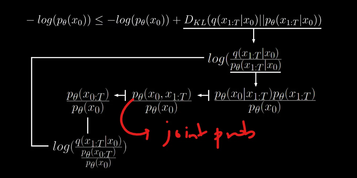
f(x) is unknown and g(x) is a known function with the condition g(x) ≤ f(x). Now, by maximizing g(x) we can say that f(x) will increase in a way because the condition needs to be satisfied. In this case, our negative log is our f(x). By subtracting KL divergence (non-negative) from function, will result in something that is less than the original function. In this case, we are minimizing KL divergence, hence the “+” symbol in the equation, so RHS will always be greater equal than LHS.

In short, a lot of the math is simplified with Bayesian rules to

After that, variational lower bound that can be minimized:
$-log(p_\theta(x_0)) \leq log(q(x_{1:T}|x_0)/p_\theta(x_{0:T}))$

Product of terms is using parameterized model $p$

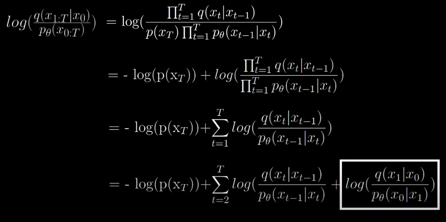
$x_{t-1}$ has a really high variance, so it is not easy to calculate based on just that, but finding out values based on $x_{t-1}$ when it is conditioned on $x_0$ provides some more context on which “direction” we can step in to denoise the image. Hence, the equations are rewritten to be conditioned on $x_0$.

This formula also has a closed form solution**.

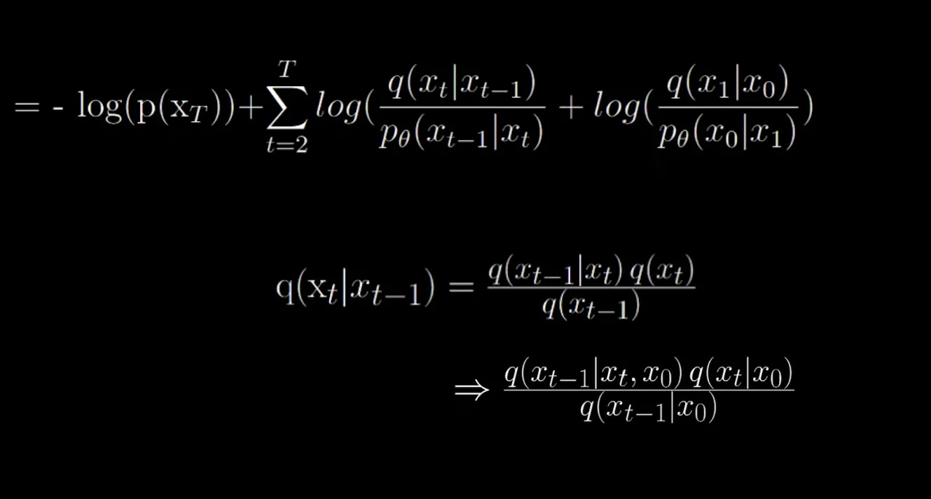
This is why t starts from 2, and the first term is removed out. If it was not removed out, and we condition the first term also on $x_0$, we would create an infinite loop since we would have $q(x_1|x_0)$ in place of $q(x_t|x_0)$ which is undesirable.

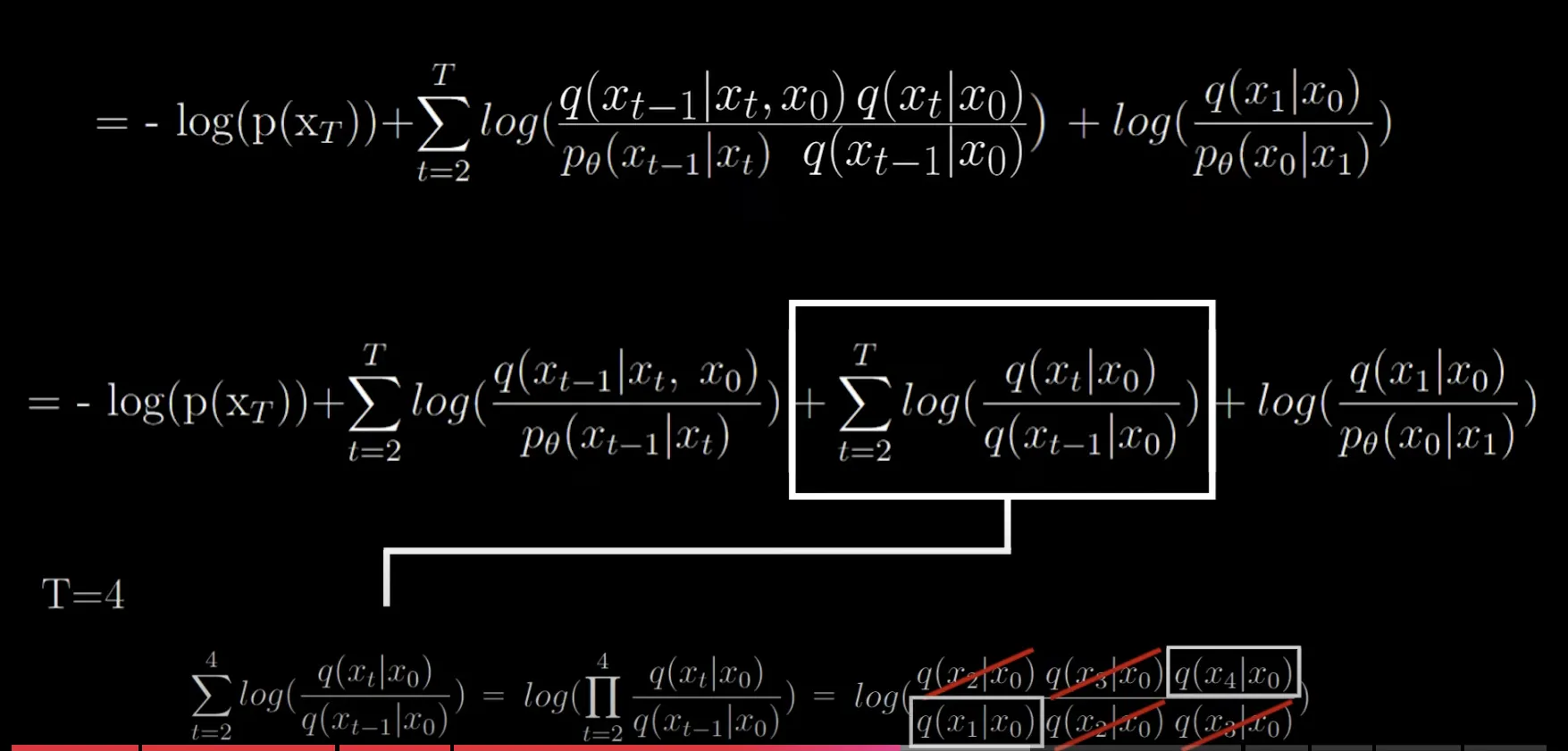
So, that summation can be simplified into: $log(q(x_t|x_0)|q(x_{1}|x_0))$

Math further simplifies into:

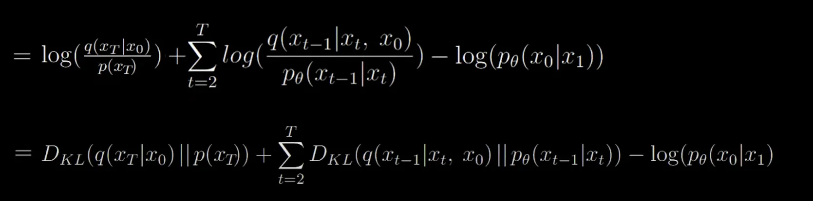
So this is in terms of KL divergence.

In terms of meaning: divergence between forward diffusion conditioned on initial image and final parameterized image + sum of divergence at every time step between the forward diffusion and corresponding reverse diffusion process of model subtracted by the

First term is constant - can be ignored

Second term: Bayes rule helped simplify the math to forward process conditioned on initial image to reverse process in the same form*. The forward process and reverse process can be seen in terms of the Gaussian sampling terms as defined before.

For the forward process, only focusing on the mean, and utilizing the closed form equation derived, we get:

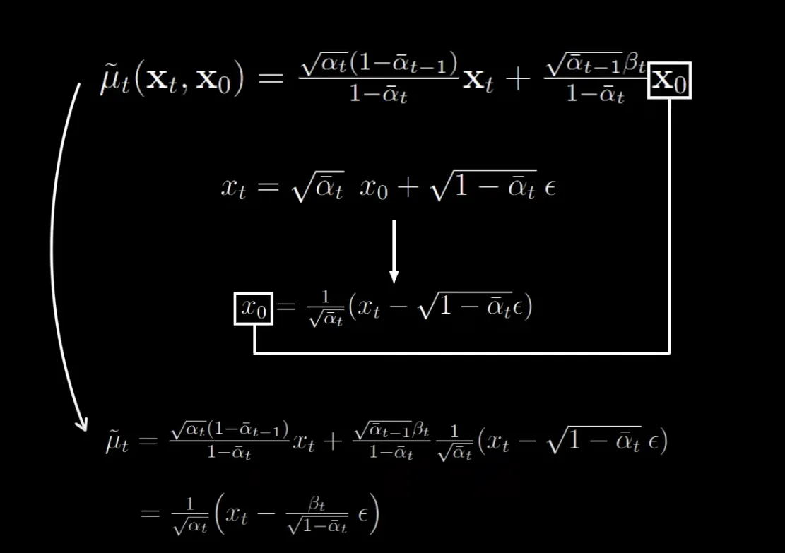
It is all simplified in the form of $x_t$ and we dont need $x_0$ anymore. It can also be seen that the mean value is just subtracting a scaled value (noise) from $x_t$ (input to the model). The $\mu$ value here is the actual or ground truth value.

For the reverse process, the $\mu$ value is a predicted value. The loss, therefore, is between the means of the forward and reverse process. It gets simplified into:

$L_t = 1/(2\sigma_t^2)||(1/\sqrt{a_t})(\beta_t/\sqrt{1-\alpha'_t})(\epsilon - \epsilon_{\theta}(x_t, t)))||^2$

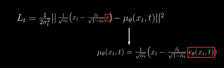
Further simplified to just the absolute mean squared difference of $\epsilon$ terms (i.e. gt - predicted) as it seemed to result in better performance.

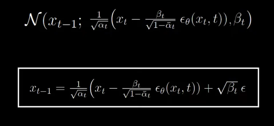
Based on the reparameterization trick, at each time step for the reverse process, $x_{t-1}$ can be caluclated as:

Last term:

I’m lost, must watch again. There is a bunch of math (you should probs rewatch)

During denoising, at t= 1, no additional random noise (second term $\sqrt{\beta_t}\epsilon$ ) is added at this final step, since this is the last denoising step and we want to fully recover the data without further corruption.

For $t > 1$ we add the second term i.e. scaled noise for the following reasons:

1. Denoising Process with Uncertainty:

• Goal: At each time step t, the model predicts and removes the noise that was added to the data in earlier steps, using the learned network $\epsilon_θ(x_t,t)$, which estimates the noise.
• Added Noise: The added noise term $\sqrt{\beta_t} \epsilon$ (with ϵ being random noise) reintroduces a small amount of randomness in the reconstruction at each time step.
• Why add noise? This reintroduced noise serves a purpose:
  • It maintains stochasticity in the denoising process, which helps the model explore different potential paths toward reconstructing the data.
  • It prevents the model from overfitting to a specific trajectory, ensuring that the denoised data at step t−1 remains a plausible sample from the data distribution.
  • The re-added noise also regularizes the model, helping it avoid collapsing to a deterministic, suboptimal reconstruction.

2. Progressive Denoising:

• Over many steps, the variance of the noise (controlled by βt) becomes smaller, meaning the randomness introduced decreases over time.
• This ensures that early steps of the diffusion process still involve significant exploration of the latent space, while later steps focus on fine-tuning and accurately reconstructing the original data.

3. Final Step t=1:

• When t=1, there's no need to add any more noise because this is the final step of the denoising process.
• At this point, the model has already learned most of the relevant information, and adding more noise would prevent an accurate recovery of the data.

Objective to optimize:

Great article with the math:

https://lilianweng.github.io/posts/2021-07-11-diffusion-models/